
THE RUNNING EXAMPLE
Welcome back! For those just joining us, we encourage you to take a look at our first post in the neural understanding series to make sure you are up to date. In that article, we described our intention to take a neural network through the various techniques of neural understanding to see if they could open up the black box of neural networks. This post will describe the working example that will be used throughout the rest of the series.
Notebooks, code, and results can be found here.
DESCRIPTION
When looking for free datasets, the first place to check was the venerable UCI ML Database.
There were several criteria for choosing the dataset:
- Computer vision-related
- Small enough to run without a GPU
- Plays well with simple networks
- Extra testing data easily acquired
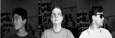
The final choice was CMU Faces, a dataset composed of graphical images of human faces. The faces are either facing left, right, up, or forward (from the subject’s perspective; subject left is camera right). The subject may be wearing sunglasses or not. Finally, the subject may be expressing an emotion: happy, sad, or neutral. The dataset exists as directories based on the subject’s username and the images are stored in PGM format. Furthermore, there are 3 different sizes to the images: 128×120, 64×60, 32×30.
The basic task of this dataset is to determine the state of the subject’s head. For this example, we chose to detect if the subject was facing left (or camera right ).

Preprocessing
Any ML enthusiast knows that all datasets need preprocessing. With that in mind, here are the steps that we took. You can find most of our process in experiments/experiment0/experiment0_create_dataset.ipynb
- The first problem that came up when using the python PIL library was that we could not open some of the pgm files. This was fixed by converting them to png files: mogrify -format png *.pgm.
- Next was to create a directory of images and a file that describes the ground truth. Again, see experiment0_create_dataset.ipynb for the code used to do this. There were three goals in mind:
- Create a classifier that would detect when the subject was looking left. Since the raw dataset encodes the pose of the subject’s face in the filename, parsing file names with the keyword ‘left’ was necessary. “1” would be stored in the ground truth file if the subject was looking to the left, “0” otherwise.
- The original dataset stores the input files in subdirectories identified by the username of the subject. To place all the input images in one directory, we generated new file names that were integer values starting from zero and incrementing for each image. These image numbers were mapped to line numbers in the ground truth file. So, image 000000.png had its ground truth stored in the first line of the ground truth file, image 000001.png had its ground truth on line 2, and so on.
- Standardize on one resolution. The original raw data had resolutions of 128×120, 64×60, or 32×30, so we rescaled all the images to 128×128 and broke aspect ratio. If breaking aspect ratio or rescaling from smaller resolutions has an impact, perhaps the neural understanding tools will help to diagnose that.
- The processed dataset can be found in datasets/face1. The file truth.csv contains the ground truths.
Training
The next thing in order is training a network on the dataset. These training processes can be found in experiments/experiment0/experiment0_create_dataset.ipynb. Some things to note:
- We created a simple network with two max pool layers sandwiched between 3 convolutional layers, two dense layers, and a dropout layer then led to a soft normalized output player.
- Since the job is to classify an image as ‘looking left’ or ‘not looking left’, the output was a 2 element vector whose elements added to 1 (softmax normalized).
- The first element describes the network’s confidence that the face was not looking left.
- The second element describes the network’s confidence that the face was looking left. Whichever position had the highest confidence was selected as the network’s decision.
- The ground truth input contains a 1 or a 0 for each image. When using categorical outputs, Keras prefers to use a ground truth encoded as [1 0] for 0, and [0 1] for 1. In other words, it prefers a ground truth with the same format as the network’s output.
- The input images were opened in grayscale mode and normalized by dividing each cell by 255.
- Finally,the sgd optimizer was used with the categorial_crossentropy loss function. The reporting metric was accuracy.
- A random 10 percent was cut out of the dataset and withheld from training for use as a testing set.
After making 10 passes (or 10 epochs) through the training data, desired results were achieved. Here are the results for a single sample run of the notebook. Multiple runs achieved similar results.
| 1685/1685 [==============================] – 29s 17ms/step – loss: 0.0318 – acc: 0.9893 test results incoming… 187/187 [==============================] – 1s 8ms/step [0.029746012331389966, 0.9946524064171123] |
After just 10 iterations, the accuracy on the training set sat at about 99%. It was initially thought that looking left would be harder to detect. Running on the testing set did even better by achieving over 99% accuracy. Wow! The model used is included in: experiments/experiment0/results/model/modela.hdf5.
Extra Testing Data
The network is now operating as intended and running the notebook several times also yielded the desired results. However, the network still needs a test run on real world data not found in the dataset. Thankfully, getting additional datasets to test is fairly easy.
- We recruited three Gravity Jack employees as test subjects: Gilbert, Ryan, and Sarah. They were told to look up, left, and right. Sunglasses or emotions weren’t part of the test so no direction was provided on that front.
- Each video was converted into a series of images using ffmpeg. The images were cropped and scaled so that they were 128×128. We used: ffmpeg -i *mp4 -vf “crop=in_w:in_w:0:(in_h-in_w)/2,scale=128:128” blank/img_%04d.png
- truth.csv was created for each set of images by hand — which turned out to be pretty fun.
The results are in datasets/testingsets/{gilbert, ryan, sarah}.

Extra Testing Results
The training results are presented in experiments/experiments0/experiment0_test_model.ipynb. Each dataset presents the value of the loss function and the reporting metric. We also count the number of false positives (images where the subject is NOT looking to their left, but the network reports the subject is looking left) and the number of false negatives (images where the subject is looking to their left but the network reports the subject is NOT looking left). Each dataset also presents 15 random false positive and 15 random false negative images. Additionally, we present the results of a typical run of the notebook.
First, let’s look at Sarah.
| 361/361 [==============================] – 3s 10ms/step [0.10927987948932198, 0.9695290859551311] false_positives: 5 false_negatives: 6 |
Wow, about 97%. That never happens. Just eleven errors. Looking at some false positives, we can see some images of her looking straight at the camera.

Let’s look at her false negatives. Clearly, she’s looking to her left.

Next, we take a look at Gilbert.
| 375/375 [==============================] – 4s 11ms/step [1.0308103105060484, 0.8666666666666667] false_positives: 0 false_negatives: 50 |
Now, 86% may sound good, but look at false negatives, 50. That is the number of positive examples in that dataset. In other words, the network does not think that Gilbert looks left, even though there’s photographic data to the contrary. Now, this is actually good news for our series on neural understanding. This is the sort of error that happens all the time in our line of work and one that neural understanding will hopefully help demystify.

Finally, we look at Ryan.
| 559/559 [==============================] – 6s 11ms/step [0.3661229715187749, 0.8372093023255814] false_positives: 20 false_negatives: 71 |
Ugh. Even worse! His false positives include some shots of him looking to his right, and his false negatives are all the images where he looks to his left. What’s going on?


What Next?
In this post, we’ve described a sample problem that might be faced in the field and produced some notebooks to run our experiments. While the networks performed well on a random split of the original dataset, they failed to work well for two out of three of our extra testing sets. The current result is a network that’s learned some concepts very well, but has trouble generalizing that concept to novel data. This is a common state of affairs in machine learning. Now, instead of guessing at problems and running experiments, we can begin to explore the tools and techniques of neural understanding to see if they offer any practical benefit!

